RFIC Design

Advance Intermodulation Distortion Analysis

This is part 2 in series of two tone intermodulation distortion analysis. Whether you are optimizing linearity or debugging it, you want to understand what are different distortion products, how do they get generated and what are they made of. For example, IM3 is made of odd order non-linearities: 3rd order has the highest contribution but 5th, 7th etc. also add to it. Another example, you might have seen IM2=2*HD2 in textbooks but when you go measure that is not the case. Why? Textbooks conveniently ignore higher order terms and just derive IM3 from 3rd order or IM2 with 2nd order assuming a weakly non-linear system. That is little wishful. We are extending the analysis to 5th order which is an optimum strike between over-analysis and under-analysis.
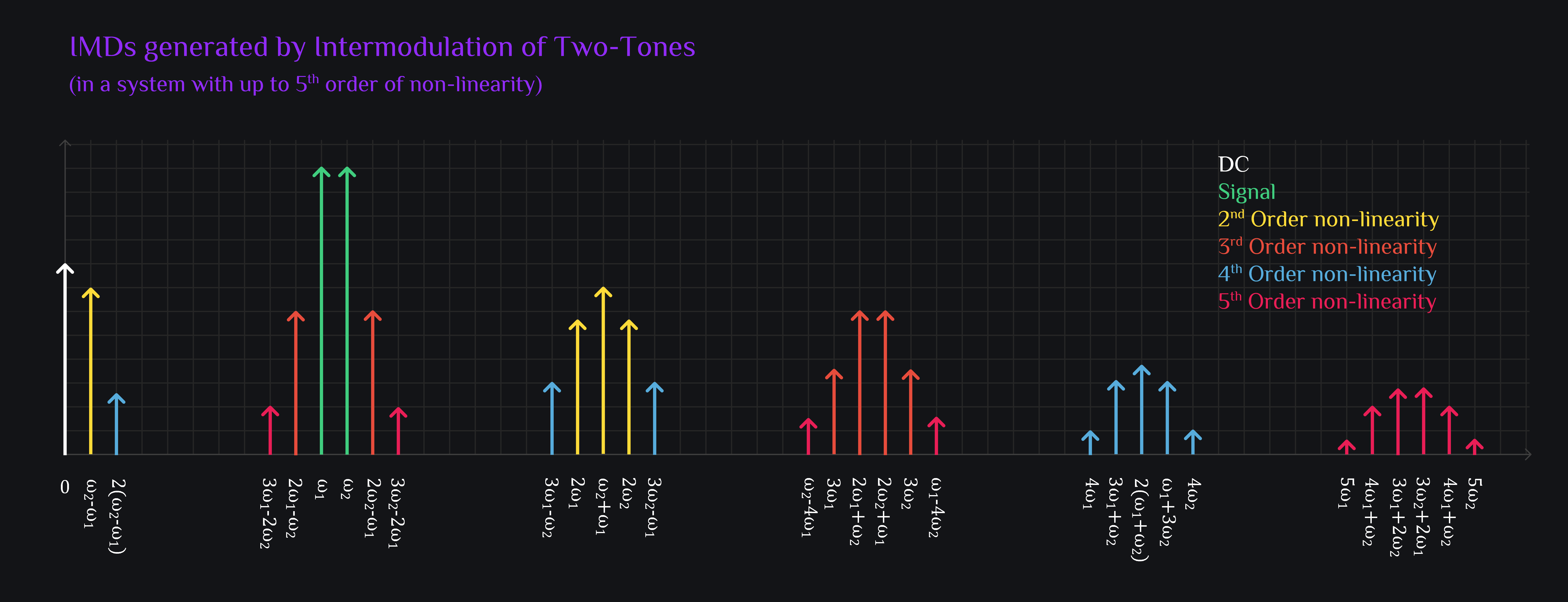
intermodulation distortion analysis of two tones up to 5th order

Intermodulation Math

Assume a non-linear memory-less system whose output has up to fifth order of non-linearity. We can relate output and input as:

$$V_{o}=a_{0}+a_{1}V_{i}+a_{2}V_{i}^2+{a_{3}V_{i}^3}+a_4V_{i}^4+a_5V_{i}^5$$

Lets excite this system with two tones: 

$$V_i=V_1cos(\omega_1t)+V_2cos(\omega_2t)$$

Output can be written as:

$$V_{o}=a_{0}+a_{1}[V_1cos(\omega_1t)+V_2cos(\omega_2t)]+a_{2}[V_1cos(\omega_1t)+V_2cos(\omega_2t)]^2+{a_{3}[V_1cos(\omega_1t)+V_2cos(\omega_2t)]^3}+{a_{4}[V_1cos(\omega_1t)+V_2cos(\omega_2t)]^4}+{a_{5}[V_1cos(\omega_1t)+V_2cos(\omega_2t)]^5}$$

Expanding Terms

Square terms:

\begin{alignat*}{6} a_{2}[V_1cos(\omega_1t)+V_2cos(\omega_2t)]^2 &=a_2V_1^2cos^2(\omega_1t)&+&a_2V_2^2cos^2(\omega_2t) &+&a_22V_1V_2cos(\omega_1t)cos(\omega_2t)\\ &=a_2V_1^2\left[\frac{1+cos(2\omega_1t)}{2}\right] &+&a_2V_2^2\left[\frac{1+cos(2\omega_2t)}{2}\right] &+&a_22V_1V_2\left[\frac{cos(\omega_1-\omega_2)t+cos(\omega_1+\omega_2)t}{2}\right] \end{alignat*}

Cubic terms:

\begin{alignat*}{6} a_{3}[V_1cos(\omega_1t)+V_2cos(\omega_2t)]^3&=a_3V_1^3cos^3(\omega_1t)&+&a_3V_2^3cos^3(\omega_2t)&+&a_33V_1^2V_2cos^2(\omega_1t)cos(\omega_2t)&+&a_33V_1V_2^2cos(\omega_1t)cos^2(\omega_2t)\\ &=a_3V_1^3\left[\frac{3cos(\omega_1t)+cos(3\omega_1t)}{4}\right] &+&a_3V_2^3\left[\frac{3cos(\omega_2t)+cos(3\omega_2t)}{4}\right] &+&a_33V_1^2V_2\left[\frac{1+cos(2\omega_1t)}{2}.cos(\omega_2t)\right] &+&a_33V_1V_2^2\left[cos(\omega_1t).\frac{1+cos(2\omega_2t)}{2}\right]\\ &=a_3V_1^3\left[\frac{3cos(\omega_1t)+cos(3\omega_1t)}{4}\right] &+&a_3V_2^3\left[\frac{3cos(\omega_2t)+cos(3\omega_2t)}{4}\right] &+&a_33V_1^2V_2\left[\frac{cos(\omega_2t)+cos(2\omega_1t)cos(\omega_2t)}{2}\right] &+&a_33V_1V_2^2\left[\frac{cos(\omega_1t)+cos(\omega_1t)cos(2\omega_2t)}{2}\right]\\ &=a_3V_1^3\left[\frac{3cos(\omega_1t)+cos(3\omega_1t)}{4}\right] &+&a_3V_2^3\left[\frac{3cos(\omega_2t)+cos(3\omega_2t)}{4}\right] &+&a_33V_1^2V_2\left[\frac{2cos(\omega_2t)+cos(2\omega_1-\omega_2)t+cos(2\omega_1+\omega_2)t}{4}\right] &+&a_33V_1V_2^2\left[\frac{2cos(\omega_1t)+cos(2\omega_2-\omega_1)t+cos(2\omega_2+\omega_1)t}{4}\right] \end{alignat*}

Quadratic terms:

\begin{alignat*}{6} a_{4}[V_1cos(\omega_1t)+V_2cos(\omega_2t)]^4 &=a_4V_1^4cos^4(\omega_1t) &+&a_44V_1^3V_2cos^3(\omega_1t)cos(\omega_2t) &+&a_46V_1^2V_2^2cos^2(\omega_1t)cos^2(\omega_2t) &+&a_44V_1V_2^3cos(\omega_1t)cos^3(\omega_2t) &+&a_4V_2^4cos^4(\omega_2t)\\ &=a_4V_1^4 \left[\frac{3+4cos(2\omega_1t)+cos(4\omega_1t)}{8}\right] &+&a_44V_1^3V_2 \left[\frac{3cos(\omega_1t)+cos(3\omega_1t)}{4}.cos(\omega_2t)\right] &+&a_46V_1^2V_2^2 \left[\frac{1+cos(2\omega_1t)}{2}\right]\left[\frac{1+cos(2\omega_2t)}{2}\right] &+&a_44V_1V_2^3 \left[cos(\omega_1t).\frac{3cos(\omega_2t)+cos(3\omega_2t)}{4}\right] &+&a_4V_2^4 \left[\frac{3+4cos(2\omega_2t)+cos(4\omega_2t)}{8}\right]\\ &=a_4V_1^4 \left[\frac{3+4cos(2\omega_1t)+cos(4\omega_1t)}{8}\right] &+&a_4V_1^3V_2 \left[\frac{3cos(\omega_1-\omega_2)t+3cos(\omega_1+\omega_2)t+cos(3\omega_1-\omega_2)t+cos(3\omega_1+\omega_2)t}{2}\right] &+&a_4\frac{3}{2}V_1^2V_2^2 \left[1+cos(2\omega_1t)+cos(2\omega_2t)+\frac{cos(2(\omega_1-\omega_2)t)}{2}+\frac{cos(2(\omega_1+\omega_2)t)}{2}\right] &+&a_4V_1V_2^3 \left[\frac{3cos(\omega_2-\omega_1)t+3cos(\omega_2+\omega_1)t+cos(3\omega_2-\omega_1)t+cos(3\omega_2+\omega_1)t}{2}\right] &+&a_4V_2^4 \left[\frac{3+4cos(2\omega_2t)+cos(4\omega_2t)}{8}\right]\\ \end{alignat*}
Pentic terms:
\begin{alignat*}{6} a_{5}[V_1cos(\omega_1t)+V_2cos(\omega_2t)]^5&=a_5V_1^5cos^5(\omega_1t)&+&a_55V_1^4V_2cos^4(\omega_1t)cos(\omega_2t)&+&a_510V_1^3V_2^2cos^3(\omega_1t)cos^2(\omega_2t)&+&a_510V_1^2V_2^3cos^2(\omega_1t)cos^3(\omega_2t)&+&a_55V_1V_2^4cos(\omega_1t)cos^4(\omega_2t)&+&a_5V_2^5cos^5(\omega_2t)\\ &=a_5V_1^5 \left[\frac{10cos(\omega_1t)+5cos(3\omega_1t)+cos(5\omega_1t)}{16}\right] &+&a_55V_1^4V_2 \left[\frac{3+4cos(2\omega_1t)+cos(4\omega_1t)}{8}.cos(\omega_2t)\right] &+&a_510V_1^3V_2^2 \left[\frac{3cos(\omega_1t)+cos(3\omega_1t))}{4}\right]\left[\frac{1+cos(2\omega_2t)}{2}\right] &+&a_510V_1^2V_2^3 \left[\frac{1+cos(2\omega_1t)}{2}\right]\left[\frac{3cos(\omega_2t)+cos(3\omega_2t))}{4}\right] &+&a_55V_1V_2^4 \left[cos(\omega_1t).\frac{3+4cos(2\omega_2t)+cos(4\omega_2t)}{8}\right] &+&a_5V_2^5 \left[\frac{10cos(\omega_2t)+5cos(3\omega_2t)+cos(5\omega_2t)}{16}\right]\\ &=a_5V_1^5 \left[\frac{10cos(\omega_1t)+5cos(3\omega_1t)+cos(5\omega_1t)}{16}\right] &+&a_55V_1^4V_2 \left[\frac{3cos(\omega_2t)}{8}+\frac{cos(2\omega_1-\omega_2)t+cos(2\omega_1+\omega_2)t}{4}+\frac{cos(4\omega_1-\omega_2)t+cos(4\omega_1+\omega_2)t}{16}\right] &+&a_55V_1^3V_2^2 \left[\frac{3cos(\omega_1t)}{4} + \frac{3cos(\omega_1-2\omega_2)t+3cos(\omega_1+2\omega_2)t}{8}+\frac{cos(3\omega_1t)}{4}+ \frac{cos(3\omega_1-2\omega_2)t+cos(3\omega_1+2\omega_2)t}{8}\right] &+&a_55V_1^2V_2^3 \left[\frac{3cos(\omega_2t)}{4} + \frac{3cos(\omega_2-2\omega_1)t+3cos(\omega_2+2\omega_1)t}{8}+\frac{cos(3\omega_2t)}{4}+ \frac{cos(3\omega_2-2\omega_1)t+cos(3\omega_2+2\omega_1)t}{8}\right] &+&a_55V_1V_2^4 \left[\frac{3cos(\omega_1t)}{8}+\frac{cos(2\omega_2-\omega_1)t+cos(2\omega_2+\omega_1)t}{4}+\frac{cos(4\omega_2-\omega_1)t+cos(4\omega_2+\omega_1)t}{16}\right] &+&a_5V_2^5 \left[\frac{10cos(\omega_2t)+5cos(3\omega_2t)+cos(5\omega_2t)}{16}\right]\\ \end{alignat*}

Collecting Terms

Color coding: DC is white, Signal is green, Square terms are yellow, Cubic orange, quadratic sky blue, and pentic red.

The All Mighty IMD Table:

\[ \begin{array}{|l|c|c|l|} \hline \text{Name} & \text{IMD Order}& \text{Frequency} & \text{Value} \\ \hline \text{DC} & 0 & \text{0} & \textcolor{#FFFFFF}{a_0}\textcolor{#FEDB39}{+\dfrac{1}{2}a_2V_1^2+\dfrac{1}{2}a_2V_2^2}\textcolor{#57ACDC}{+\dfrac{3}{8}a_4V_1^4+\dfrac{3}{8}a_4V_2^4+\dfrac{3}{2}a_4V_1^2V_2^2} \\ \hline \hline \text{Beat/Envelope} & 2 &\omega_2-\omega_1 & \textcolor{#FEDB39}{a_2V_1V_2}\textcolor{#57ACDC}{+\dfrac{3}{2}a_4V_1^3V_2+\dfrac{3}{2}a_4V_1V_2^3} \\ \hline \text{HD2 of Envelope} & 4 &2(\omega_2-\omega_1) & \textcolor{#57ACDC}{\dfrac{3}{4}a_4V_1^2V_2^2} \\ \hline \text{Left IM5} & 5 &3\omega_1-2\omega_2 & \textcolor{#E91E56}{\dfrac{5}{8}a_5V_1^3V_2^2} \\ \hline \text{Left IM3} & 3 &2\omega_1-\omega_2 & \textcolor{#E74C3C}{\dfrac{3}{4}a_3V_1^2V_2}\textcolor{#E91E56}{+\dfrac{15}{8}a_5V_1^2V_2^3+\dfrac{5}{4}a_5V_1^4V_2} \\ \hline \text{Signal Tone1} & 1 &\omega_1& \textcolor{#40CE7F}{a_1V_1}\textcolor{#E74C3C}{+\dfrac{3}{4}a_3V_1^3+\dfrac{3}{2}a_3V_1^2V_2}\textcolor{#E91E56}{+\dfrac{5}{8}a_5V_1^5+\dfrac{15}{4}a_5V_1^3V_2^2+\dfrac{15}{8}V_1^4V_2} \\ \hline \text{Signal Tone2} & 1 &\omega_2& \textcolor{#40CE7F}{a_1V_2}\textcolor{#E74C3C}{+\dfrac{3}{4}a_3V_2^3+\dfrac{3}{2}a_3V_1V_2^2}\textcolor{#E91E56}{+\dfrac{5}{8}a_5V_2^5+\dfrac{15}{4}a_5V_1^2V_2^3+\dfrac{15}{8}V_1V_2^4} \\ \hline \text{Right IM3} & 3 &2\omega_2-\omega_1 & \textcolor{#E74C3C}{\dfrac{3}{4}a_3V_1V_2^2}\textcolor{#E91E56}{+\dfrac{15}{8}a_5V_1^3V_2^2+\dfrac{5}{4}a_5V_1V_2^4} \\ \hline \text{Right IM5} & 5 &3\omega_2-2\omega_1 & \textcolor{#E91E56}{\dfrac{5}{8}a_5V_1^2V_2^3} \\ \hline \text{IMD4} & 4 &3\omega_1-\omega_2 & \textcolor{#57ACDC}{\dfrac{1}{2}a_4V_1^3V_2} \\ \hline \text{HD2 of Tone1} & 4 &2\omega_1 & \textcolor{#FEDB39}{\dfrac{1}{2}a_2V_1^2}\textcolor{#57ACDC}{+\dfrac{1}{2}a_4V_1^4+\dfrac{3}{2}a_4V_1^2V_2^2} \\ \hline \text{IMD2} & 2 &\omega_1+\omega_2 & \textcolor{#FEDB39}{a_2V_1V_2}\textcolor{#57ACDC}{+\dfrac{3}{2}a_4V_1^3V_2+\dfrac{3}{2}a_4V_1V_2^3} \\ \hline \text{HD2 of Tone2} & 4 &2\omega_2 & \textcolor{#FEDB39}{\dfrac{1}{2}a_2V_2^2}\textcolor{#57ACDC}{+\dfrac{1}{2}a_4V_2^4+\dfrac{3}{2}a_4V_1^2V_2^2} \\ \hline \text{IMD4} & 4 &3\omega_2-\omega_1 & \textcolor{#57ACDC}{\dfrac{1}{2}a_4V_1V_2^3} \\ \hline \text{IMD5} & 5 &4\omega_1-\omega_2 & \textcolor{#E91E56}{\dfrac{5}{16}a_5V_1^4V_2} \\ \hline \text{3rd Harm of Tone1} & 3 &3\omega_1& \textcolor{#E74C3C}{\dfrac{1}{4}a_3V_1^3}\textcolor{#E91E56}{+\dfrac{5}{16}a_5V_1^5+\dfrac{5}{4}a_5V_1^3V_2^2} \\ \hline \text{IMD3} & 3 &2\omega_1+\omega_2 & \textcolor{#E74C3C}{\dfrac{3}{4}a_3V_1^2V_2}\textcolor{#E91E56}{+\dfrac{15}{8}a_5V_1^2V_2^3+\dfrac{5}{4}a_5V_1^4V_2} \\ \hline \text{IMD3} & 3 &2\omega_2+\omega_1 & \textcolor{#E74C3C}{\dfrac{3}{4}a_3V_1V_2^2}\textcolor{#E91E56}{+\dfrac{15}{8}a_5V_1^3V_2^2+\dfrac{5}{4}a_5V_1V_2^4} \\ \hline \text{3rd Harm of Tone2} & 3 &3\omega_2& \textcolor{#E74C3C}{\dfrac{1}{4}a_3V_2^3}\textcolor{#E91E56}{+\dfrac{5}{16}a_5V_2^5+\dfrac{5}{4}a_5V_1^2V_2^3} \\ \hline \text{IMD5} & 5 &4\omega_2-\omega_1 & \textcolor{#E91E56}{\dfrac{5}{16}a_5V_1V_2^4} \\ \hline \text{HD4 of Tone1} & 4 &4\omega_1 & \textcolor{#57ACDC}{\dfrac{1}{8}a_4V_1^4} \\ \hline \text{IMD4} & 4 &3\omega_1+\omega_2 & \textcolor{#57ACDC}{\dfrac{1}{2}a_4V_1^3V_2} \\ \hline \text{IMD4} & 4 &2(\omega_1+\omega_2) & \textcolor{#57ACDC}{\dfrac{3}{4}a_4V_1^2V_2^2} \\ \hline \text{IMD4} & 4 &3\omega_2+\omega_1 & \textcolor{#57ACDC}{\dfrac{1}{2}a_4V_1V_2^3} \\ \hline \text{HD4 of Tone2} & 4 &4\omega_2 & \textcolor{#57ACDC}{\dfrac{1}{8}a_4V_2^4} \\ \hline \text{HD5 of Tone1} & 5 &5\omega_1 & \textcolor{#E91E56}{\dfrac{1}{16}a_5V_1^5} \\ \hline \text{IMD5} & 5 &4\omega_1+\omega_2 & \textcolor{#E91E56}{\dfrac{5}{16}a_5V_1^4V_2} \\ \hline \text{IMD5} & 5 &3\omega_1+2\omega_2 & \textcolor{#E91E56}{\dfrac{5}{8}a_5V_1^3V_2^2} \\ \hline \text{IMD5} & 5 &3\omega_2+2\omega_1 & \textcolor{#E91E56}{\dfrac{5}{8}a_5V_1^2V_2^3} \\ \hline \text{IMD5} & 5 &4\omega_2+\omega_1 & \textcolor{#E91E56}{\dfrac{5}{16}a_5V_1V_2^4} \\ \hline \text{HD5 of Tone2} & 5 &5\omega_2 & \textcolor{#E91E56}{\dfrac{1}{16}a_5V_2^5} \\ \hline \end{array} \]
They way you should read this table is: “Okay, I am debugging beat term. Let’s see what it is made of. You look at the second row of table and realize it is a sum of 2nd and 4th order terms. You also see 4th order term has bigger scalers (3/2) than 2nd order term. I see, so maybe I should check my circuit and see what is generating 4th order term. Maybe I can optimize that instead of just looking at 2nd order term.”

Numerical Example

Let’s put things in perspective. We took a CMOS transistor, excited it with some input voltage and looked at the output current to see relative distortion levels (yes we are looking at gm non-linearity). It gave us following:

\[ \begin{array}{|c|c|c|c|} \hline \text{Co-efficient} & \text{Linear}& \text{dBc} & \text{Sign} \\ \hline \textcolor{#40CE7F}{a_1} & 1& 0 & + \\ \hline \textcolor{#FEDB39}{a_2} & 0.0562& -25 & + \\ \hline \textcolor{#E74C3C}{a_3} & 0.01& -40 & - \\ \hline \textcolor{#57ACDC}{a_4} & 0.0018& -55 & - \\ \hline \textcolor{#E91E56}{a_5} & 0.001& -60 & + \\ \hline \end{array} \]

It says, in a typical circuit, you would get -25dBc HD2, -40dBc HD3, -55dBc HD4 and -60dBc HD5 (without optimization of course, just raw typical numbers). We derive our polynomial coefficients from these, and now we have an idea of typical values of a1,a2,a3,a4 and a5 in a non-linear system. Also note the signs, typically our circuits are compressive which means when you input big sin wave, output looks more like a square wave, and you know for a square wave (composed of cosines) you have 3rd harm out of phase with fundamental, and 5th harm is in phase (that is what our table also says in the “sign” column). Signs for even terms are very subjective, they can be anything really.

Let’s take these co-efficients and insert in our “The All Mighty IMD Table” to have a visual picture of relative levels of IMDs.
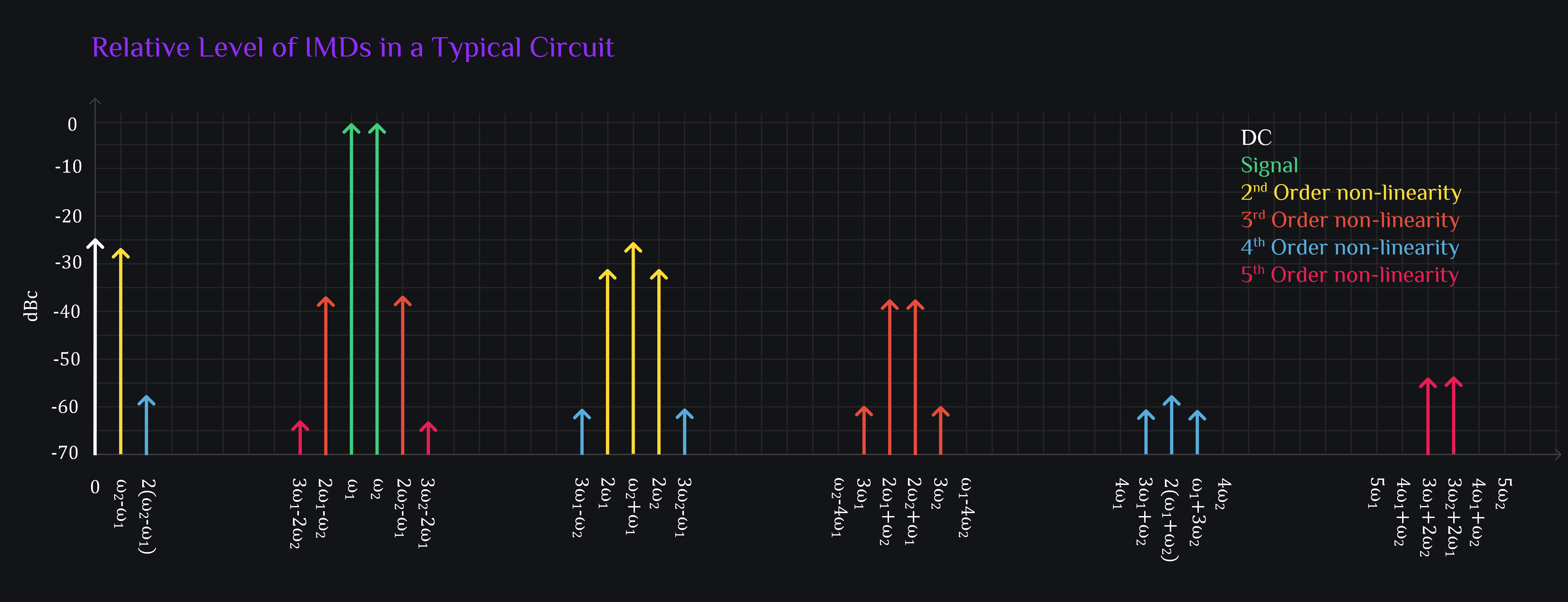
typical levels of intermods in a circuit

We filtered out tones below -70dBc in above image (just to unclutter). What you should worry about is that HD2s and beat terms are even bigger than IM3 in a typical system, and similarly IMD4 products are bigger than IM5s. That means even order non-linearities are greater than odd order, but it so happened that odd order fell close to your signal and became more critical because you always said you could filter out far-flung even order terms. Well, that may not always be the case. Consider a very wideband system:
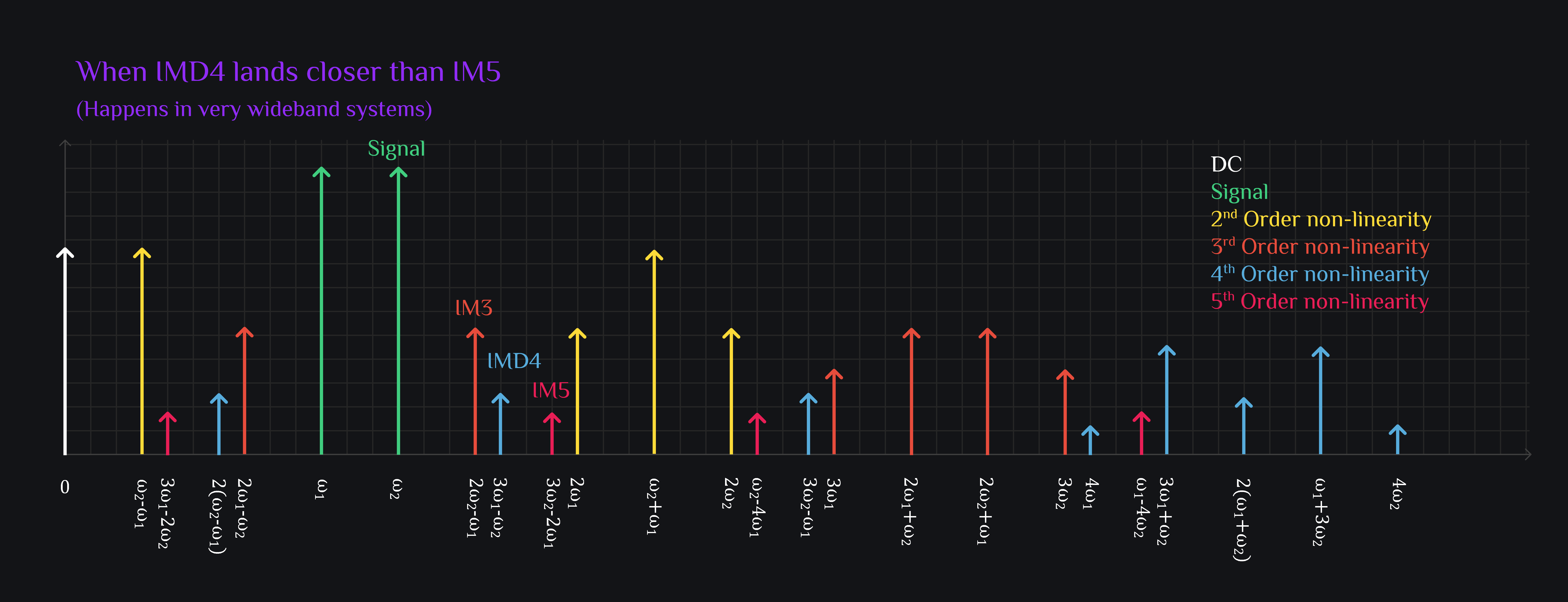
typical intermods in a wideband system

When you start spacing out signal tones, non-linearities start spreading out, thus coming closer to your desired signal. Above image shows that IMD4 landed between IM3 and IM5. So now you need to optimize for IMD4 (or at least keep this guy in mind) in addition to IM3 and IM5. We must remark that this scenario happens for very wideband systems (e.g., say 2.7GHz center RF frequency, and signal bandwidth from 2.4GHz to 3GHz (that’s fractional BW of 22%!), in this case IMD4 lands on IM5). 


Another insight you can get from this numerical example:

$$IM3=HD3+9.5\;dB \text{ (that is what your textbook said)}$$ $$IM3 = HD3 + 13.7\;dB \text{ (that is what we got)}$$ $$IM2=HD2+6\;dB \text{ (that is what your textbook said)}$$ $$IM2 = HD2 + 6.4\;dB \text{ (that is what we got)}$$

Why did this happen? Because textbook ignored higher order terms. We didn’t (well we ignored very high order terms, gotta stop at some point right?). Download our spreadsheet below for this numerical example.

Intermods Calculator

Author: RFInsights 
Date Published: 05 Jan 2023
Last Edit: 02 Feb 2023