A Journey from Resonance to Impedance Matching
Chp. 1: Origin of Q-Factor
The Deadly Beginnings
#1 When a Capacitor discharges through Resistor
Let’s start from a capacitor C. Charge it to 1V. Now connect it to a resistor R. What will happen? Capacitor will lose charge exponentially. You would say, ok, my time constant \(\tau\) is RC, so in about 5\(\tau\) seconds, my capacitor would have lost it all because that’s how an exponential function goes.
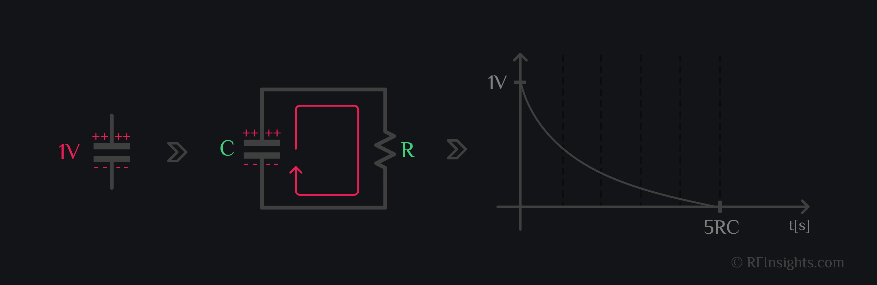
Ever wonder though why did it have to be an exponential function? Why couldn’t it be linear or some other function for that matter? Asking such questions is important to build upon fundamentals. The way current is drawn from the capacitor depends on the load connected to it. A resistor is such a load which demands from the capacitor to send the charge in a way that rate of change of charge is equal to charge itself at any point in time. Let’s do some math to see this.
What is something whose derivative is equal to its current value? Think about it. It’s an exponential function.
Therefore, the charge (or the derivative of charge which is current) decays exponentially. A resistor will always draw current from the capacitor exponentially. Story changes for an inductor.
#2 When a Capacitor discharges through an Inductor
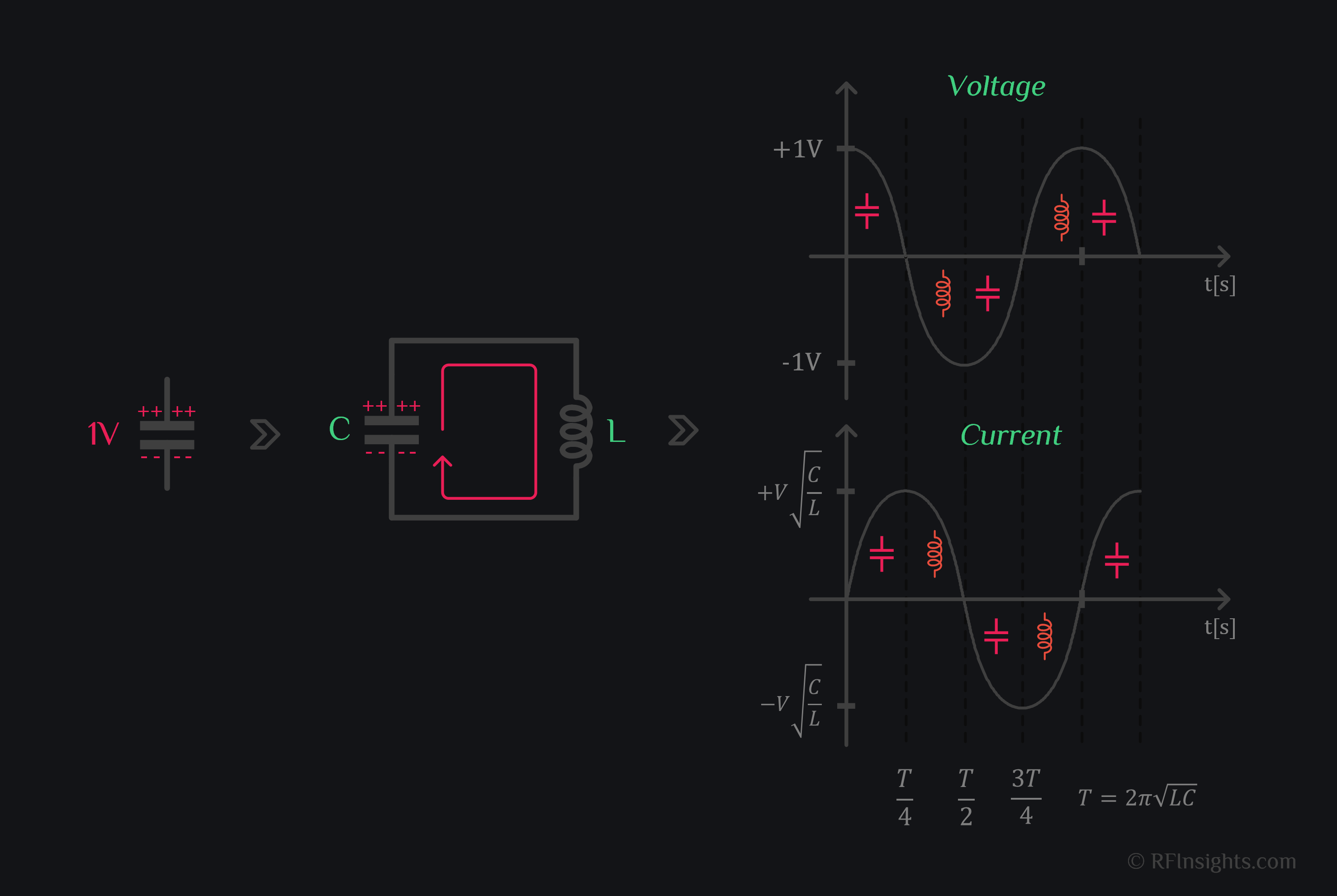
Let’s start again from a capacitor C. Charge it to 1V. Now connect it to an inductor L. What will happen? Capacitor will lose charge in a sinusoid fashion.
When you connect this charged capacitor to an inductor, the capacitor will start losing its charge, so the voltage would start decreasing Current would start flowing and inductor will begin to expand its magnetic field. When the capacitor has lost it all (at T/4), and there is no charge to flow, current would have collapsed to zero except that inductor resists the sudden change in current (because of back EMF). So, the inductor keeps the current flowing in same direction and capacitor starts getting charge from inductor, and charges with opposite polarity now. A time (T/2) comes when inductor has lost it all (magnetic field has collapsed) and all the charge is transferred to capacitor. Capacitor will discharge through inductor again, then inductor discharges through capacitor again, and this goes on. The cycle repeats. We call this behavior resonance, and the LC tank as resonator.
The questions arise:
- Why is it sinusoid though, why couldn’t it be something else say a triangular waveform?
- What is the time period of this energy exchange? How fast does capacitor gets discharged now?
Therefore, the charge on capacitor (or voltage as V=Q/C) is exchanged with inductor in a cosine fashion, and the time period of this exchange is T/4 (meaning 4 charge exchanges happened in one cycle)
How fast is the charge exchange in LC compared to RC? Assume R=C=L=1, the charge on capacitor would decay in 5 sec for RC and \(\frac{\pi}{2}\) sec for LC which is about \(\pi\) times faster than RC!
#3 When a Capacitor Discharges through Resistor and Inductor
#3.1 Qualitative Explanation
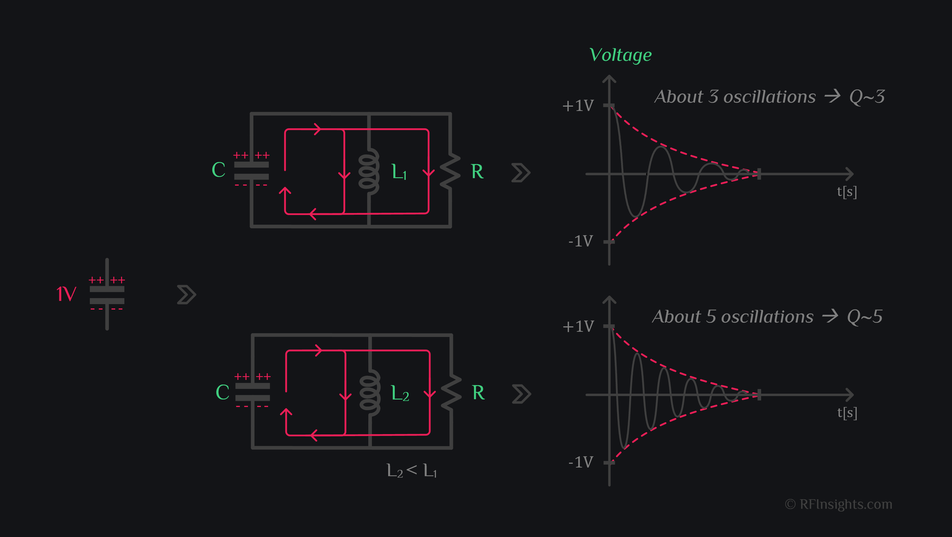
Let’s go back again. Charge the capacitor C to 1V. Connect it to a resistor R and inductor L. What will happen? Capacitor will exchange charge with inductor again in a sinusoid fashion except that resistor will demand the charge exponentially. Energy exchange may go on for a couple cycles until the resistor has dissipated all the charge away . We would call this a bad quality resonator which couldn’t sustain resonance. I think you are getting an idea where we are heading. Let’s keep developing our thought:
If we were to compare two resonators say L1C and L2C where L1>L2, say both have a resistor R in parallel to them. Do both these resonators have same quality (after all R is same)? No. Turns out that L2C is a better resonator than L1C (L2C sustained more oscillations). So, then that’s how folks started quantifying resonators. Look at how many oscillations, and that is the quality factor of a resonator (well sort of, not very precise, but visually if you were to look at a resonator response, you would just count the number of cycles it sustained oscillation, and that would be your approximate Q factor of circuit, and this is happens to be an interview question)
Ok, visually we can determine Q-factor by looking at number of cycles. But how should we quantify it mathematically? Is there a way by looking at RLC values, we could tell the quality of a resonator? That is what folks also felt and ended up discovering Q=R/X relation. Here’s how it would have happened:
So, for resonator to be a good quality or let’s say have at least one cycle of oscillation, we would say, hey 5RC time of charge decay in a pure RC should be greater than T0 time of oscillation in a pure LC. This way we would make sure that at least one cycle of back and forth charge transfer between capacitor and inductor happened before resistor could lose it all away. Let’s write that down mathematically:
This tells us that if \(\omega_0\)RC is equal to one, we could hope to see at least one oscillation (because we would have ensured 5RC decay is longer than one oscillation time period). If it is two, we would see two oscillations. That’s it. We have arrived at our metric of Quality for resonators. The term \(\omega_0\)RC is what we can call as quality factor. You don’t need to count cycles now. Just evaluate \(\omega_0\)RC for resonator and that will be the number of cycles your resonator is going to survive. A little manipulation reveals, that \(\omega_0\)RC is actually a ratio of R and X.
So, quality of a resonator depends on all, R & C & L. It’s not just R, or RC time constant or LC resonance frequency. Everything put together in above expression is your measure of Quality. Now you can also appreciate why L2 in above example gave higher Q than L1. This concludes our discussion on how the term Quality factor originated, how was it used to compare resonators by looking at number of cycles, and how did those cycles ended up being equal to R/X.
#3.2 Quantitative Explanation
(Caution: Lots of math coming, good if it has been long and you want to refresh couple things, best if you really want to see things through, bad if you are like young me who didn’t appreciate math)
Let’s try to derive response of a parallel RLC tank. We can write currents as:
This is a second order linear homogenous differential equation with constant coefficients.
- Linear because it has a variable and its derivative, both present in this equation.
- Homogenous because each term is only related to one variable or its derivative.
- Constant co-efficient because \(\omega_0\) and Q are constants.
Linear homogenous differential equations with constant coefficients can be reduced to characteristic equations and solve algebraically as follows:
where K1 and K2 can be found through initial conditions. At t=0, we had capacitor charged to 1V (let’s say Vo to make it generic). Let’s put that in.
At t=0, the inductor had zero current flowing through. Let’s put that in.
Put this in (1), we get our K1 and K2
Let’s plug these in our general solution, and simplify to see a more plausible form of V(t):
Plug these in equation above:
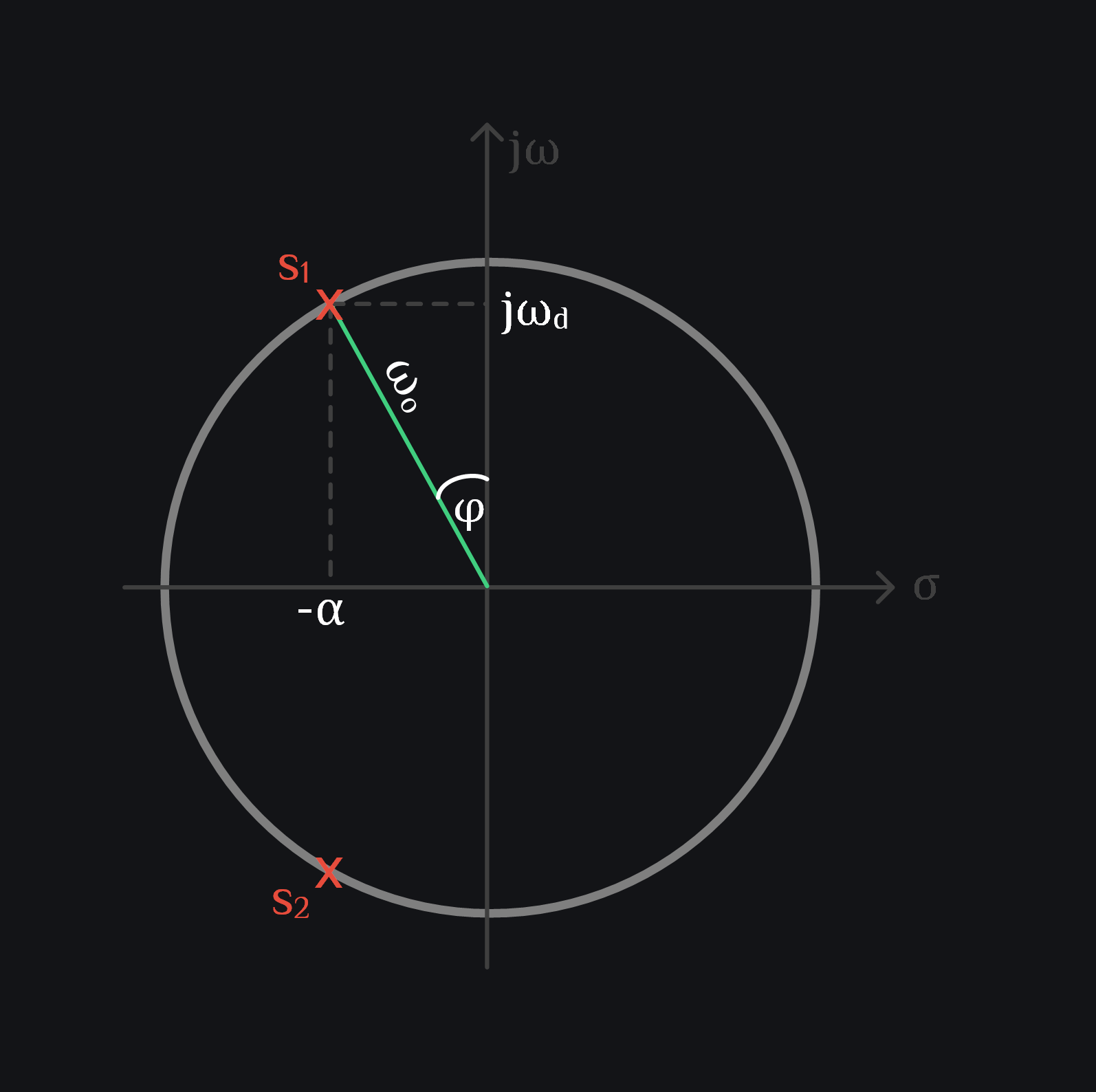
and finally, we have done it, we have our rigorous math exercise telling us exactly the same thing: your RLC is a resonator, oscillating at frequency \(\omega_{d}\) (which is lesser than \(\omega_o\)), with a starting phase of \(\phi\), and amplitude is scaled by a decaying exponential.
Also interesting to note that, in pure RC, voltage dies out in 5RC seconds, but in RLC, voltage dies out in 10RC.
#3.3 Precise Relation between Q and Number of Cycles
We said that Q is approximately equal to number of cycles it takes for your voltage to die out with time. Let’s figure out the exact relation between Q and number of cycles N.
For exponential e-t to die out, we consider t=5 to be sufficient time (remember 5 time constants in case of RC). So our, cosine will die out when:
This is the precise relation between Q and N. Q is equal to 1.6 number of cycles. So for example, if Q is 5, you should see about 8 cycles of oscillation before it is all vanished.
We inserted V(t) equation in Desmos, go ahead and play with Q factor below, count the number of cycles.
#4 Origin of Classical Definition of Q
To close the topic, let’s now try to understand the origin of classical definition of Q (saying Q equals energy stored over energy destroyed). To do that, we need a little bit of more math. Bear with us. Let’s nail this down while we are at it. Current through capacitor can be written as:
Plug V(t) expression of Eq. (2) in
We know, at resonance, inductor and capacitor currents are out of phase for parallel RLC (like cap current is -jI, ind current is +jI, thus 180 out of phase). Therefore, we can give inductor current by removing negative sign of capacitor current:
Now, energy in the tank at any point in the time can be given as:
Rate of change of energy is power, so the power dissipated in the resistor can be given as:
(note -ive sign because energy decays with time)
Re-arranging the above equation takes us to the physical definition of Q
This is the classical definition of Q factor, and now we see how was it derived, and why did the factor 2\(\pi\) appear. It didn’t need to be there because one can already get an idea of the quality of a resonator by just dividing the energy stored by energy destroyed but the factor of 2\(\pi\) was added so that the math aligns (as you saw in derivation above that it just showed up).
We inserted W(t) and Q equations in Desmos graphing calculator below. You can see QF matches with Q (see expressions list in graph below) saying that yes energy stored over energy destroyed multiplied by 2\(\pi\) is indeed equal to Q. Go ahead and play with Q slider in the graph below to see how stored and lost energies move.
Also, you might wonder, ok I get that energy stored vs energy lost idea but I just want to know how much power is destroyed from starting point. Let’s say I have x power at beginning of cycle, how much would I be left at the end of cycle. Answer is straightforward, you know now it dies out exponentially.
For Q=10, this evaluates to be 53.3 % which means after each cycle you would be left with 53.3% of power at the start of that cycle.
Browse by Tags
RFInsights
Date Published: 09 Feb 2023
Last Edit: 09 Feb 2023