A Journey from Resonance to Impedance Matching

Chp. 6: Quality Factor and Bandwidth

Q-factor is Inverse of 3dB BW. Design or Coincidence?

You have seen this

Q = \frac{1}{FBW}

where FBW is fractional bandwidth $\dfrac{\Delta \omega}{\omega_o}$ and $\Delta \omega$ represents 3dB bandwidth around your resonance frequency $\omega_o$.

We tried looking this up on internet that how come Quality factor and Bandwidth are inversely related, and even if they were how come 3dB bandwidth comes out exactly equal of inverse of Q. Everyone throws this around as one of the “definition/formula” of quality factor not explaining how could anyone have conjured this all up. After all, the one and only true definition of quality factor is energy stored over energy loss, that is the origin of the term Quality factor, rest of the definitions are (or better should be) derived from this. This motivated us to look deep into Quality factor and bandwidth derivation and dig out some fundamental intuitions around it, and hence this article.

Q-Factor and Bandwidth Derivation from Classical Q-Factor Formula

Take an RLC tank. Say it resonates at frequency w_o and has Q-factor of Q_o. Change L up and down keeping C fixed, resonance frequency changes up and down, and Q of tank also changes linearly. Energy stored in an LC tank equals to 0.5CV² any point in time (capacitor and inductor’s energy vary over time because they exchange between themselves but their sum remains same). Similarly, average power dissipated remains same because R didn’t change. Therefore, ratio $\frac{E_S}{P_D}$ does not change with resonance frequency, and hence the linear dependence of Q on f as shown in image below.

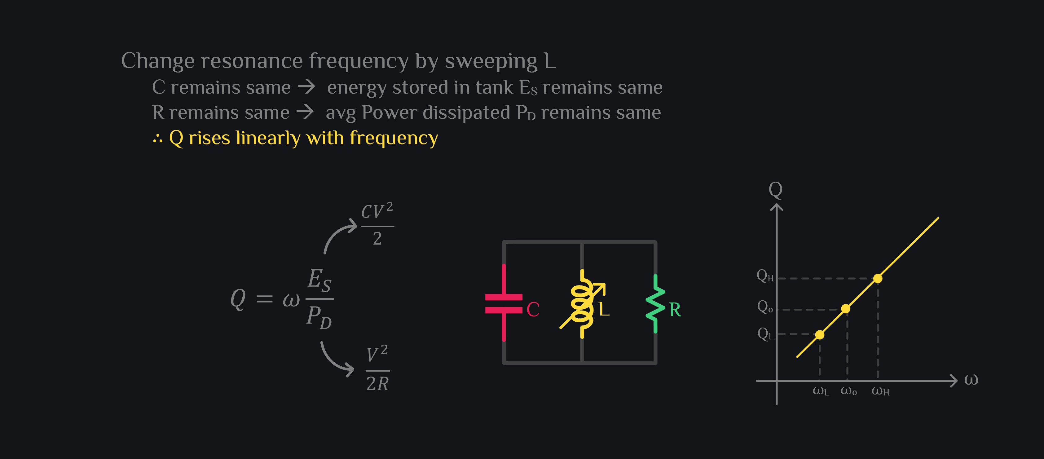
Now let’s change C up and down keeping L fixed, resonance frequency changes again down and up respectively, and Q changes too (this time by $\frac{1}{f}$ fashion though because reactance of capacitor changes by $\frac{1}{f}$ fashion)

The point of this exercise is to realize that Q and frequency indeed have a relation. Let’s put the two curves on top of each other as shown in right image. We observe for a $\Delta \omega$, there is a $\Delta Q$ indicating that there is a relation between bandwidth and quality factor – that’s our cue. Let’s focus on yellow curve for now and write this down in math:

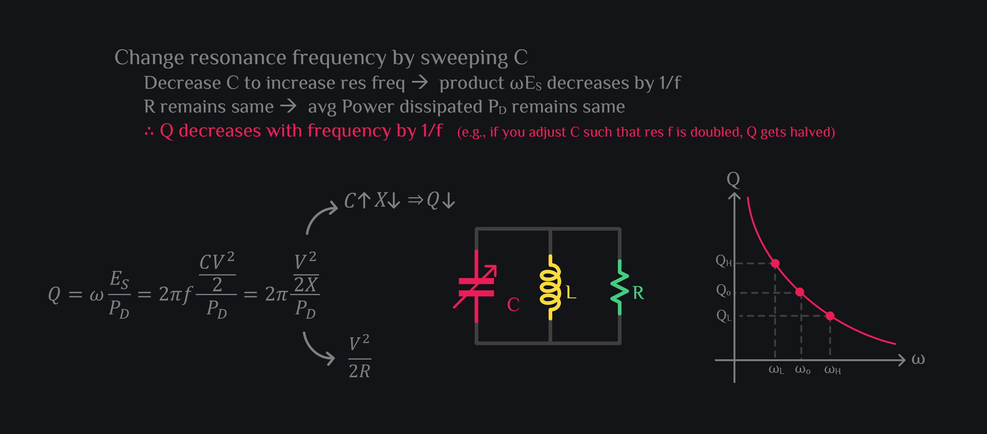
(yellow because math is easier, $\frac{E_S}{P_D}$ remains same over frequency as we mentioned before, the math of red curve is in appendix and leads to same conclusion what we are going to draw below).

Q_o = \omega_o \frac{E_S}{P_D};\;\;\;Q_H = \omega_H \frac{E_S}{P_D};\;\;\;Q_L = \omega_L \frac{E_S}{P_D}$$ $$ Q_H - Q_L = (\omega_H - \omega_L) \frac{E_S}{P_D}$$ $$\Delta Q = \Delta \omega \frac{E_S}{P_D}$$ $$\Delta Q \times \omega_o= \Delta \omega \frac{E_S}{P_D} \times \omega_o$$ $$\Delta Q \times \omega_o= \Delta \omega \times Q_o$$ $${\LARGE \textcolor{#40CE7F}{\frac{\Delta Q}{Q_o} = \frac{\Delta \omega}{\omega_o}}}\;\;\; (1)

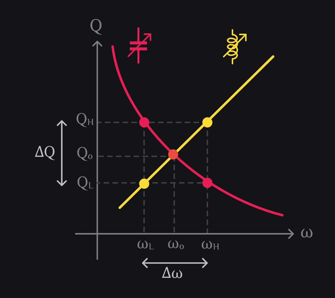
This gives us interesting insight that your bandwidth relative to your center frequency is equal to change in Q relative to Q at center frequency. If you allow $\Delta Q$ to be bigger, you can get wider bandwidth. Or if you decrease Q_o, you get wider bandwidth too. This answers our first question that how bandwidth and quality factor turned out to be inversely related, and that this relation was hidden inside the classical Q-factor formula itself.

Now to the 2^nd question: how come $\Delta \omega$ turned out to be 3dB BW and not some x dB? Was it by design or a pure coincidence that our beloved half power bandwidth concept naturally landed as being equal to inverse of Q (and we mean not just proportional to inverse of Q but exactly equal to inverse of Q). To understand this, think of parallel RLC tank. When does power drop by 3dB? When current through resistor goes down to 0.707I where I was the current at resonance. For current to drop to this level, X of the tank needs to be equal to R (don’t be fooled by reactance – you might think X=R will lead to half half current division, that is not correct, because X never draws current in phase with R, so there is always a chance that R could get more from source even though X=R, if it were two Rs, then yes they draw same amount of current from source at same time (means in phase) so source current has to get divided half and half). Ok, so for 3dB power, we can write that tank susceptance needs to be equal to tank conductance:

|B_L - B_C| = G $$ $$\left|\frac{B_L}{G} - \frac{B_C}{G}\right| = 1$$ $$\left|\frac{R}{X_L} - \frac{R}{X_C} \right| = 1$$ $$|Q_L - Q_C| = 1 $$ $$\Delta Q = 1

This says the frequencies where the difference between tank reactances gets equal to tank resistance or in other words, where $\Delta Q$ gets equal to 1, are 3dB frequencies. Insert this in Eq. (1)

\frac{1}{Q_o} = \frac{\Delta \omega}{\omega_o}$$ $${\LARGE \textcolor{#40CE7F}{Q_o = \frac{\omega_o}{\Delta \omega} = \frac{1}{FBW}}}

This answers our second question that $\Delta \omega$ is not just any bandwidth but actually 3dB BW when $\Delta Q$ is one, and with that the inverse of Q is exactly equal to fractional BW.

But wait we are not home free yet. There is a piece of puzzle that we missed. We took the results of $\Delta Q=1$ from an RLC tank where we didn’t vary LC, instead we changed frequency, and we applied this to Eq. (1) which was actually derived for resonant tanks (meaning we varied either L or C to keep the tank in resonance as we changed frequency). Does it make sense? Yes, it turns out you whether you change LC values or you change frequency, Q behaviors are same. Let’s look at the right image again. We said before if you were to change L, you move resonance frequency and Q, and you get yellow curve. If you move C, you get red curve. But these curves look very similar to reactance behavior over frequency; if you were to just change frequency (keeping L&C same), and look at the Q of inductor, and Q of capacitor, you will exactly land on the yellow and red curve respectively. So $\Delta Q$ of LC (where you didn’t change LC but frequency) for some $\Delta \omega$ is equal to $\Delta Q$ of LC (where you changed LC to change the frequency) for same $\Delta \omega$. This might seem a little overwhelming, so take your time to grasp this, but even if you can’t wrap your mind around it it, don’t worry, these are nitty gritty details for nerds us, not really needed in today’s circuit design. Go on read below, and come back to this later.

Why Leftside 3dB BW is Lower than Rightside 3dB BW?

Ever wonder when you plot a resonator response across frequency, you do not see equal BW to right and left side of resonance frequency. The left side is always lower. For example, we took an RLC resonator with 2GHz resonance frequency and Q-factor of ~1.6. You can see lower 3dB frequency is ~1.47GHz (0.53GHz lower than 2GHz) whereas higher frequency is 2.72GHz (0.72GHz higher than 2GHz, thus higher BW on right side).

This has to do with capacitor. We said 3dB BW occurs when tank X becomes equal R. Tank X is basically delta between ind X and cap X. Notice how quickly this delta grows on the left side of resonance because of $\frac{1}{f}$ behavior of capacitor’s reactance. On the other hand, delta grows slowly on right side because capacitor’s reactance decay slows down (again $\frac{1}{f}$ behavior). This gives right side advantage, and it takes more frequencies for delta to grow equal to R on right side, thus giving more BW at right side. Think of series RLC circuit. Image below plots ind reactance X_L, cap reactance X_C, their delta X_L-X_C, and how fast this delta grows $\frac{d}{df} (X_L-X_C)$. Y-axis is R of the RLC, and x-axis is frequency. You can see if Q of the tank is big (i.e., R is small e.g., R=1), the reactance delta (orange color) takes almost same frequencies left and right to become equal to R. If Q is small (look at R=10), you can see reactance delta becomes quickly equal to R=10 on left side (thus lesser BW on left) but takes more frequencies at right side (thus higher BW on right).

It is interesting to note that if capacitor behaved linearly with frequency, that is if $X_C= -2 \pi fC$, then left and right side BW would have been equal. A negative inductor can do that. So if you knew why this left and right side BWs were different, and if they mattered that much in your system, you would quickly have thought of how can design you design a negative inductor, because that will solve your problem. If you didn’t know, you wouldn’t think of negative inductor as well. That is why we dive deep into these articles. Innovation lies in strong fundamentals, not complex circuits.

Why Center Frequency is Geometric Mean of 3dB Frequency?

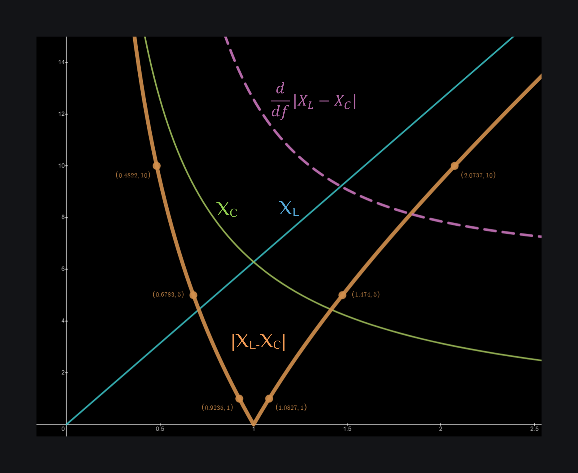
To a layman, arithmetic mean (your regular average) makes most sense. If you were given that $\omega_H$ and $\omega_L$ are your 3dB frequencies, and asked what is the center frequency you would be inclined to say its $\frac{\omega_H+\omega_L}{2}$ but it turns out its actually $\sqrt{\omega_H \omega_L}$. The former is called arithmetic mean, and latter is called geometric mean. So the question is why did it have to be geometric mean? To understand this, look reactance delta in above image again. Let’s pick some points for different R values.

$$R=1 \implies (0.9235,1) \;\;\;\text{&}\;\;\; (1.0827,1)$$ $$R=5 \implies (0.6783,1) \;\;\;\text{&}\;\;\; (1.474,1)$$ $$R=10 \implies (0.4822,1) \;\;\;\text{&}\;\;\; (2.0737,1)$$

What can you say about central tendency of this data set? If you take arithmetic mean of these points, it would come out different for each pair but you take geometric mean, it would come out equal to 1 which is correct as you can see visually in above image too. This means the central point of this data is geometric mean.

R=1 \implies (0.9235,1) \;\;\;\text{&}\;\;\; (1.0827,1) \implies AM =1.003 \;\;\; \text{&} \;\;\; GM=1$$ $$R=5 \implies (0.6783,1) \;\;\;\text{&}\;\;\; (1.474,1) \implies AM =1.076 \;\;\; \text{&} \;\;\; GM=1$$ $$R=10 \implies (0.4822,1) \;\;\;\text{&}\;\;\; (2.0737,1) \implies AM =1.278 \;\;\; \text{&} \;\;\; GM=1

But then again, why did this happen? Answer: because of capacitor’s reactance $\frac{1}{f}$ behavior with frequency. The reactance delta of tank is given as:

X_L - X_C$$ $$\omega L - \frac{1}{\omega C}

Let’s see how fast this delta changes with frequency. Take derivative of it:

\frac{d}{d\omega} \left(\omega L - \frac{1}{\omega C}\right) \implies \left[L + \frac{1}{C}\frac{1}{\omega^2}\right]

This shows that reactance delta grows by $\frac{1}{f^2}$, that is at every next frequency the new value of reactance delta is given by this much times of previous value rather than this much addition on previous value. And that is a characteristic of geometric series, hence the center frequency ends up being geometric mean, and that is also why if you look at resonator response at x times higher or x times lower frequency than resonance, you would see it develops same amplitude. But you if you were to look at resonator response at +x frequency and -x frequency from resonance frequency, you would find different amplitude.

Formal Non-Intuitive Derivation

For record, let’s just derive it in a pure mathematical too. Recall from above:

Q_o = \omega_o \frac{E_S}{P_D};\;\;\;Q_H = \omega_H \frac{E_S}{P_D};\;\;\;Q_L = \omega_L \frac{E_S}{P_D}$$ $$ Q_HQ_L = \omega_H \omega_L \frac{E_S^2}{P_D^2}$$ $$ \omega_o^2 \times Q_HQ_L = \omega_o^2 \times \omega_H \omega_L \frac{E_S^2}{P_D^2}$$ $$ \omega_o^2 \times Q_HQ_L = \omega_H \omega_L \times Q_o^2 $$ $$ \omega_o^2 \times \frac{R}{X_H}\frac{R}{X_L} = \omega_H \omega_L \times \frac{R^2}{X_o^2} $$ $$ \omega_o^2 \times \frac{1}{\omega_H L}\frac{1}{\omega_L L} = \omega_H \omega_L \times \frac{1}{\omega_o^2 L^2} $$ $$\implies \omega_o^2 = \omega_H \omega_L$$ $$\implies {\LARGE \textcolor{#40CE7F}{\omega_o = \sqrt{\omega_H \omega_L}}}

Having developed the insights behind Quality factor and Bandwidth, the situation is now ripe to proceed to matching networks – a topic for next chapter.

Appendix

Derivation of Quality factor and Bandwidth relation from Capacitor’s reactance (red curve)

Q_o = \omega_o \frac{E_S}{P_D};\;\;\;Q_H = \omega_H \frac{E_S}{P_D};\;\;\;Q_L = \omega_L \frac{E_S}{P_D}$$ $$ Q_H - Q_L = \frac{1}{P_D} \left[ \omega_H E_H - \omega_L E_L \right] $$ $$ Q_H - Q_L = \frac{1}{P_D} \left[\omega_o E_S \frac{\omega_o}{\omega_H} - \omega_o E_S \frac{\omega_o}{\omega_L} \right] \;\;\; \text{(because if you increase f by x, tank's Q and thus } \omega_o E_s \text{ drops by } \frac{f_o}{x} \text{ )}$$ $$ \Delta Q = \omega_o \frac{E_S}{P_D}\omega_o \left[\frac{1}{\omega_H}-\frac{1}{\omega_L}\right]$$ $$ \Delta Q = Q_o \omega_o \left[\frac{\omega_L-\omega_H}{\omega_H \omega_L}\right]$$ $$ \frac{\Delta Q}{Q_o} = \omega_o \left[\frac{\Delta \omega}{\omega_o^2}\right]$$ $$ \frac{\Delta Q}{Q_o} = \frac{\Delta \omega}{\omega_o}

Excel File

RFInsights

Published: 09 March 2023
Last Edit: 09 March 2023